DEVELOPER'S WEB LOG
Fasterer Atmospheric Rendering
August, 4 2019
So there’s been an improvement to atmospheric scattering that I want to share. You’ll want to make sure to read Alan Zucconi’s series on scattering if you’re not familiar with the topic. Also read the earlier blog post on Fast atmosphere scattering to get yourself acquainted with the problem I’m dealing with.
We’re basically trying to solve this integral:
`I = int_A^L exp(-(sqrt(x^2 + z^2) - R)/H) dx`

Like many integrals, it has no closed form solution. We have to make approximations.
I’ve come to learn a few people have worked on this problem before. Christian Schüler was the first person I’m aware of. He wrote a chapter of a book that described an approximation for what’s known as the “Chapman function”. The Chapman function is a related concept. It effectively measures the relative density of particles in the atmosphere, just like we’re doing, however it does so using a different method signature. Rather than work with 2d cartesian coordinates relative to the center of the world, it works with viewing angle and altitude. I’ve found this method signature to be less convenient to work into a classical raymarch algorithm, since for every step of the raymarch I have to calculate an angle relative to the zenith for that step. For that reason I’ve never gotten around to implementing it.
The approximation I made last time doesn’t have that problem, but I couldn’t escape the nagging feeling that it lacked mathematical elegance. The problem it was trying to prevent was a division by zero. The division by zero occurred when you naïvely solved the integral using integration by substitution:
`int_A^L exp(-(sqrt(x^2 + z^2) - R)/H) dx approx -H sqrt(x^2 + z^2)/x exp((sqrt(x^2 + z^2) - R)/H)`
There was a distance function used to calculate height, and when you swapped it out for a stretched-out quadratic height approximation, you could make sure that division by zero never occurs in the region of interest. But that required defining a region of interest, so we setup some arbitrary fractions a and b from which the slope and intercept for the quadratic approximation could be sampled.
And that’s why it felt so ugly. You had to pick some value for the magic constants a and b, they had to work well together, and they had to work well for every planet in the universe.
So I kept revisiting the problem, more than I probably should have, and eventually I was able to reason my way to a better solution.
My first insight was to reduce the number of parameters to consider. I realized that if all distances (both input and output) were expressed in scale heights, we could do away with H:
`int_A^L exp(R-sqrt(x^2 + z^2)) dx approx -sqrt(x^2 + z^2)/x exp(R-sqrt(x^2 + z^2))`
I then thought about what would happen in certain situations. When `z=R` and `x=0`, the behavior for height:
`h(x,z,R) = sqrt(x^2 + z^2) - R`
begins to resemble a parabola:
`h(0,R,R) approx approx x^2 - R`
in which case the integral is proportionate to the error function:
`int_A^L exp(R-x^2) dx propto 1/2 sqrt(pi) e^R erf(x)`
And we know from Schüler's work that the limit to our integral as `x->oo` is described by the chapman function when viewing the horizon:
`Ch|| = (1/(2(z-r)) + 1) sqrt((pi (z-r)) / 2)`
So we can refine our estimate to:
`Ch|| erf(x)` where `z=R` and `x=0`
however if `z=0` then height is linear:
`h = abs(x) - R`
in which case the integral is trivial:
`int_A^L exp(R - x) dx = -exp(R - x)`
We need some way to switch between these two integral solutions seamlessly. We first notice that if we attempt a naïve solution using integration by substitution:
`int_A^L exp(R - sqrt(x^2 + z^2)) dx approx - 1/(h') exp(h(x)) approx - sqrt(x^2 + z^2)/x exp(R - sqrt(x^2 + z^2))`
we see that the division by zero occurs when `x=0`. That only appreciably occurs when `z=R`. So whatever workaround we use to address the division by zero ought to in these circumstance return the approximation from the error function instead of the bogus results from the naïve integration by substitution.
So how about this: we "nudge" the derivative by some amount (let's call it `F`) to prevent division by zero when `x=0`.
`int_A^L exp(R - sqrt(x^2 + z^2)) dx approx - 1/(x/sqrt(x^2 + z^2) + F) exp(R - sqrt(x^2 + z^2))`
When the ray only grazes the planet, `F` should be exactly what's needed to spit out the known good answer, `Ch|| erf(x)`. Since `erf(x)` is close enough to `-exp(R-sqrt(x^2+z^2))`, we'll say:
`F approx 1/(Ch||) = 1 / ((1/(2x) + 1) sqrt((pi x) / 2))` when `x=0` and `z=R`
When the ray strikes head on (`z=0`), the amount we nudge it by should be zero.
`F = 0` when `z = 0`
So all we need is to modify `Ch||` in such a way that F goes to 0 for large values of `x`. We'll call this modification `Ch` I started by calculating `I` using numerical integration and evaluating the expression that was equivalent to `Ch`:
`Ch = (-exp(-h) / I - h')^-1`
After some trial and error, I found `Ch approx sqrt(pi/2 (x^2 + z))` works to a suitable approximation, but for those who want more accuracy for a little less performance, it's best to simply to add a linear term onto `Ch||`:
`Ch approx (1/(2 sqrt(x^2+z^2))+1) sqrt(1/2 pi z) + ax`
where I set `a = 0.6`
So in other words, all we're really doing is a modified integration by substitution using the "o-plus" operation between `1/h'` and `Ch|| + ax` to prevent division by zero.
`I = int_A^L exp(R-sqrt(x^2 + z^2)) dx approx (1/h' oplus Ch) exp(R-sqrt(x^2 + z^2))`
O-plus turns out to be pretty useful for preventing division by 0, in general.
So chances are you’ve clicked a link here wanting to see the code. Well, here it is:
// "approx_air_column_density_ratio_along_2d_ray_for_curved_world"
//   calculates the distance you would need to travel
//   along the surface to encounter the same number of particles in the column.
// It does this by finding an integral using integration by substitution,
//   then tweaking that integral to prevent division by 0.
// All distances are recorded in scale heights.
// "a" and "b" are distances along the ray from closest approach.
//   The ray is fired in the positive direction.
//   If there is no intersection with the planet,
//   a and b are distances from the closest approach to the upper bound.
// "z2" is the closest distance from the ray to the center of the world, squared.
// "r0" is the radius of the world.
float approx_air_column_density_ratio_along_2d_ray_for_curved_world(
    float a,
    float b,
    float z2,
    float R
){
    // GUIDE TO VARIABLE NAMES:
    //  capital letters indicate surface values, e.g. "R" is planet radius
    //  "x*" distance along the ray from closest approach
    //  "z*" distance from the center of the world at closest approach
    //  "R*" distance ("radius") from the center of the world
    //  "h*" distance ("height") from the center of the world
    //  "*0" variable at reference point
    //  "*1" variable at which the top of the atmosphere occurs
    //  "*2" the square of a variable
    //  "d*dx" a derivative, a rate of change over distance along the ray
    float X  = sqrt(max(R*R -z2, 0.));
    float div0_fix = 1./sqrt((X*X+sqrt(z)) * 0.5*PI);
    float ra = sqrt(a*a+z2);
    float rb = sqrt(b*b+z2);
    float sa = 1./(abs(a)/ra + div0_fix) *     exp(R-ra);
    float sb = 1./(abs(b)/rb + div0_fix) *     exp(R-rb);
    float S  = 1./(abs(X)/R  + div0_fix) * min(exp(R-sqrt(z2)),1.);
    return sign(b)*(S-sb) - sign(a)*(S-sa);
}

// "approx_air_column_density_ratio_along_2d_ray_for_curved_world"
//   calculates column density ratio of air for a ray emitted from the surface of a world to a desired distance,
//   taking into account the curvature of the world.
// It does this by making a quadratic approximation for the height above the surface.
// The derivative of this approximation never reaches 0, and this allows us to find a closed form solution
//   for the column density ratio using integration by substitution.
// "x_start" and "x_stop" are distances along the ray from closest approach.
//   If there is no intersection, they are the distances from the closest approach to the upper bound.
//   Negative numbers indicate the rays are firing towards the ground.
// "z2" is the closest distance from the ray to the center of the world, squared.
// "r" is the radius of the world.
// "H" is the scale height of the atmosphere.
float approx_air_column_density_ratio_along_2d_ray_for_curved_world(
    float x_start,
    float x_stop,
    float z2,
    float r,
    float H
){
    float X = sqrt(max(r*r -z2, 0.));
    // if ray is obstructed
    if (x_start < X && -X < x_stop && z2 < r*r)
    {
        // return ludicrously big number to represent obstruction
        return BIG;
    }
    float sigma =
        H * approx_air_column_density_ratio_along_2d_ray_for_curved_world(
            x_start / H,
            x_stop  / H,
            z2      /(H*H),
            r       / H
        );
    // NOTE: we clamp the result to prevent the generation of inifinities and nans,
    // which can cause graphical artifacts.
    return min(abs(sigma),BIG);
}

// "try_approx_air_column_density_ratio_along_ray" is an all-in-one convenience wrapper
//   for approx_air_column_density_ratio_along_ray_2d() and approx_reference_air_column_density_ratio_along_ray.
// Just pass it the origin and direction of a 3d ray and it will find the column density ratio along its path,
//   or return false to indicate the ray passes through the surface of the world.
float approx_air_column_density_ratio_along_3d_ray_for_curved_world (
    vec3  P,
    vec3  V,
    float x,
    float r,
    float H
){
    float xz = dot(-P,V);           // distance ("radius") from the ray to the center of the world at closest approach, squared
    float z2 = dot( P,P) - xz * xz; // distance from the origin at which closest approach occurs
    return approx_air_column_density_ratio_along_2d_ray_for_curved_world( 0.-xz, x-xz, z2, r, H );
}
Fast Atmospheric Rendering
March, 24 2019
There have been some major changes recently to the appearance of the simulation. I’ve gone through great pains to learn physical rendering techniques in an effort to eventually model how atmospheric compounds affect climate. Those two topics might not sound interrelated, but it turns out they share a lot of the same equations.
What I want to discuss today is one particular aspect of this new rendering model: atmospheric scattering. Zoom into a planet really close and you’ll see how the atmosphere forms a haze:
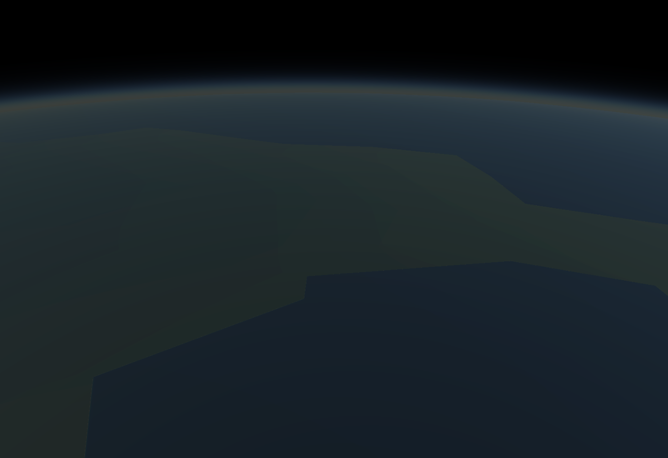
How does it do this? Well, it’s a long story, and I won’t describe it in full detail. There are already plenty of resources available online that teach you how it’s done. I highly recommend reading Alan Zucconi’s series on atmospheric scattering, if you’re interested in the topic.
I pretty much use the same technique as Alan Zucconi, but there is one significant improvement I made that I want to talk about. This was an improvement I made to combat performance issues when rendering with multiple light sources. Tectonics.js has a nifty feature where it samples light sources from across several points in time. This is done to create a “timelapse” effect when running at large timesteps.
I didn’t want to toss out this feature in order to implement atmospheric scattering, but I have to admit: it’s a pretty usual requirement for an atmospheric renderer. Most of the time, atmospheric renderers assume there is only one light source, that being the sun. You could trivially modify an atmospheric renderer to run on multiple light sources, but let’s consider the performance implications of doing so.
Atmospheric renderers use raymarching to find something known as the column density along a path from the viewer to the light source. You might see this mentioned here as the “column density ratio.” When we say this, we mean the column density expressed relative to the density of air on the surface of the planet. Most standard atmospheric renderers are implemented as follows:

for each point "A" along the view ray "V":
  for each point "B" from A to light source "L":
    sum up the column density ratio
You will notice the implementation above uses two nested for loops. What if we added support for multiple light sources? We would need to add another for loop:

for each point "A" along the view ray "V":
  for each light source "L":
    for each point "B" from A to light source "L":
      sum up the column density ratio
We now have three nested for loops, each of which might run about 10 iterations in our use case. We’re looking at something on the order of 1000 calculations. That’s 1000 calculations for every pixel, for every frame. This is madness.
So is there anyway we can pare this down? Can we eliminate one of the for loops?
Well, fortunately for us, this code is not very well optimized. We need to consider what we’re doing here: we’re summing up the mass that’s encountered along a series of infinitesimally small steps from “A” to “L”. In essence, we’re calculating an integral.
To be more precise: we’re trying to find the integral of density from points “A” to “L”.
The integral looks like this:
`int_A^L rho(x) dx`
Here the density `rho` is defined by the Barometric formula
`rho(x) = exp(-(h(x))/H)`
where `H` is the scale height of the planet, and height `h` is defined by the distance formula minus the planet's radius `R`
`h(x) = sqrt(x^2 + z^2) - R`
Here, `x` represents some distance along the ray relative to the closest approach, and `z` represents the distance to the center of the planet when at that closest approach (see diagram on the left)
So all together, we’re trying to solve:
`int_A^L exp(-(sqrt(x^2 + z^2) - R)/H) dx`
Solve this integral, and you will be able to completely eliminate a nested for loop from your raymarching algorithm. That’s a factor of 10 performance improvement!
If this were a college calculus course, you might think to use integration by substitution. This results in the following expression:
`-H/(h'(x)) exp(-(h(x))/H)`
However this produces bogus results when the ray just barely grazes the planet, such that `z approx R` and `x approx 0`. This is because the height changes very little in these circumstances, so `h'(x) = 0`. In essence, we divide by 0, and results near this singularity will look unrealistic.
Fortunately, we only need something that looks convincing, so we can afford to make approximations. All we need is a good approximation for height whose derivative never reaches 0. I've tried several approaches, but the best I've found so far uses a quadratic approximation for height. It's derivative still eventually reaches 0, but you can stretch out the approximation by some factor `a` to ensure it never gets anywhere near 0 for any positive value of x.
`h(x) approx 1/2 a h''(x_b) + h'(x_b) + h(x_b)`
Here, `x_b` is a sample point along the path through the atmosphere. If `x_0` is the point at which we encounter the surface, and `x_1` is the point at which we encounter some arbitrary "top" of the atmosphere, then `x_b` can be thought of as a point between them, defined by a fraction b:
`x_b = x_0 + b(x_1-x_0)`
For my implementation, I define the "top" of the atmosphere to be 6 scale heights from the surface. Under these circumstances, I set `b = 0.45` and `a = 0.45`. I find this gives pretty good approximations for column density ratio given virtually any realistic value of `z` or `H`. See for yourself: follow the link here and adjust the sliders for `H` and `z` and see how close the appoximation (red) gets to the actual column density (black)
Lastly, if you’re interested in borrowing some of my code, check out raymarching.glsl.c in the Tectonics.js source code, or just copy/paste the code below:
float approx_air_column_density_ratio_along_2d_ray_for_curved_world(
    float x_start, // distance along path from closest approach at which we start the raymarch
    float x_stop,  // distance along path from closest approach at which we stop the raymarch
    float z2,      // distance at closest approach, squared
    float r,       // radius of the planet
    float H        // scale height of the planet's atmosphere
){
    float a = 0.45;
    float b = 0.45;

    float x0 = sqrt(max(r *r -z2, 0.));
    // if ray is obstructed
    if (x_start < x0 && -x0 < x_stop && z2 < r*r)
    {
        // return ludicrously big number to represent obstruction
        return 1e20;
    }

    float r1      = r + 6.*H;
    float x1      = sqrt(max(r1*r1-z2, 0.));
    float xb      = x0+(x1-x0)*b;
    float rb2     = xb*xb + z2;
    float rb      = sqrt(rb2);
    float d2hdx2  = z2 / sqrt(rb2*rb2*rb2);
    float dhdx    = xb / rb;
    float hb      = rb - r;
    float dx0     = x0          -xb;
    float dx_stop = abs(x_stop )-xb;
    float dx_start= abs(x_start)-xb;
    float h0      = (0.5 * a * d2hdx2 * dx0      + dhdx) * dx0      + hb;
    float h_stop  = (0.5 * a * d2hdx2 * dx_stop  + dhdx) * dx_stop  + hb;
    float h_start = (0.5 * a * d2hdx2 * dx_start + dhdx) * dx_start + hb;

    float rho0  = exp(-h0/H);
    float sigma =
        sign(x_stop ) * max(H/dhdx * (rho0 - exp(-h_stop /H)), 0.)
      - sign(x_start) * max(H/dhdx * (rho0 - exp(-h_start/H)), 0.);

    // NOTE: we clamp the result to prevent the generation of inifinities and nans,
    // which can cause graphical artifacts.
    return min(abs(sigma),1e20);
}

// "approx_air_column_density_ratio_along_3d_ray_for_curved_world" is just a convenience wrapper
//   for the above function that works with 3d vectors.
float approx_air_column_density_ratio_along_3d_ray_for_curved_world (
    vec3  P, // position of viewer
    vec3  V, // direction of viewer (unit vector)
    float x, // distance from the viewer at which we stop the "raymarch"
    float r, // radius of the planet
    float H  // scale height of the planet's atmosphere
){
    float xz = dot(-P,V);           // distance ("radius") from the ray to the center of the world at closest approach, squared
    float z2 = dot( P,P) - xz * xz; // distance from the origin at which closest approach occurs
    return approx_air_column_density_ratio_along_2d_ray_for_curved_world( 0.-xz, x-xz, z2, r, H );
}
Upcoming Blog Post Storm
March, 21 2019
Things have been going on with the model and I haven’t had time to describe it all. Some of the things that were implemented this past year are pretty innovative. Just to give a summary:
- An on-rails orbital mechanics model that can derive average insolation for any solar system over timespans ranging from seconds to millions of years.
- A physically based tectonics model that derives plate velocity from the density of oceanic crust.
- A climate model that provides realistic estimates for air temperature in less than a millisecond for any point on the surface of a planet
- A fast, physically realistic atmospheric scattering system that entirely eliminates a costly nested raymarch loop using a closed form approximation
- A physically based rendering engine
I need to create a series of blog posts to document these features and how they were implemented: what resources helped me, what I did different, what it delivered. In order to do so I need to change my style a bit: less well polished, more down to the point. The idea is simply to write all this stuff before I forget it.
More to come.
Version 2.0
September, 16 2017
More than a year ago a feature request was filed on the Tectonics.js project repository. The request called for more visualizations within the model: crust age, mineral composition, and other cool features. This was something that I had wanted to implement for a long time. Crust age plays a big role in determining the density of oceanic crust, which in turn determines the motion of tectonic plates. Modeling crust age would be easy enough - simply add a new property to your rock column object and increment its value every update cycle. So I started with crust age. I setup the visualization and ran the simulation.
Then I saw the results.
Ho boy. This wasn’t what I expected.
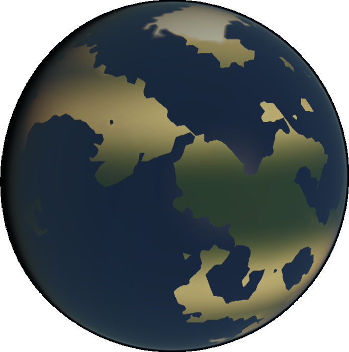
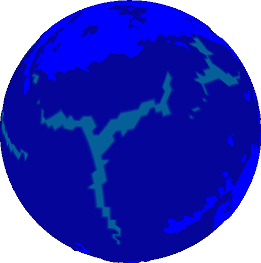
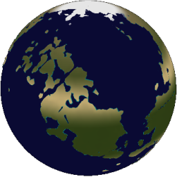
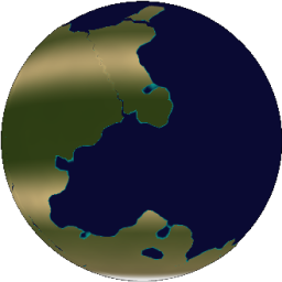
Take these results and compare them with Earth. The same colors are used to represent age.
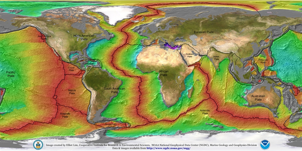
Notice anything different? The map of Earth is red. That means the ocean crust on Earth is much younger.
As a matter of fact, you’ll be hard pressed to find any ocean crust on Earth that’s older than 250 million years. This has to do with how the ocean crust responds to age. When ocean crust ages, it cools. When something cools, it becomes dense. When something becomes more dense than the liquid that surrounds it, it sinks. Sinking things drag down the other things they’re attached to. Things like tectonic plates. You can now start to see how this causes tectonic plates to move.
Now back to Tectonics.js. Look at virtually any simulation and you find ocean crust that’s well past this age, perhaps a billion years old or more. It isn’t too hard to find the reason. It comes down to what Tectonics.js was doing at its very core:
- generate a series of plates at random
- generate a series of velocities at random
- destroy crust whenever intersections occur
This is how its done in virtually every other non-academic tectonics simulator I’ve seen, and it’s wrong. There is simply no way you can reproduce Earth’s age distribution this way. Earth’s age distribution isn’t something you can reproduce by tweaking parameter values. The problem lies with the model itself.
I tried for a long time to solve the age problem with incremental change. Maybe you could keep your random plate geometry, but set the velocity to collide with nearby old crust? Maybe your plates could follow a predetermined path, one that maximizes their coverage of the globe? I spent several months trying these things off and on: considering them, designing them, implementing them, testing them. The experience left me deeply disheartened.
In an act of desperation, I took a new approach. Rather than start with the model and use it to produce the right output, I would start with the right output and then use it to produce the model.
An entire year passed as I redesigned the model from the ground up. I started the project as an experiment. I make a lot of experimental branches and most go nowhere. To outsiders, it probably looked like the project was abandoned, but truth is, I think this was one of the most productive years I’ve spent on the model.
The model that resulted was far removed from the original. Sure, the graphics look the same, but the internals were upended. Nothing was left untouched. I could only think of one way to describe it:
Version 2.0
Version 2.0 was such a change that I even debated creating a new website for it, but version 2.0 is so much better than the original that I don’t want to leave any uncertainty among the users:
Version 1.0 is a joke. Version 2.0 is the thing to use.
Only version 2.0 has an architecture that is flexible enough to implement all the things you ever dreamed of: atmospheric models, hydrological models, biosphere models, anything. Only version 2.0 uses the same mathematical framework that geophysicists use to model tectonics academically.
The Outset
I started out with one mantra, like a psychotic killer:
ocean crust must die.
If ocean crust is older than a certain threshold, it’s gone. No exceptions. Its like the Logan’s Run of oceanic crust. The model can keep old ocean crust in memory if it likes, but the pressure brought about by its sinking has to cause newer adjacent crust to take its place. Once it’s covered, it’s gone.
But how do you accomplish that? Well, nature does it somehow. So how does nature do it?
Over long periods of time, Earth’s crust behaves as a fluid, like a cup ouf cold pitch.
It seems like the perfectly correct answer involves some sort of fluid simulation. In case you’re wondering, no I don’t do fluid simulation. I don’t implement the Navier Stokes equation within the model. I just don’t have the computational power to do so. But I do use the same mathematical framwork. That framework is vector calculus. Its objects are scalar fields and vector fields.
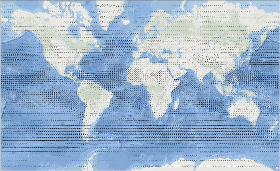
What is a field? You already know what a field is. You see them in maps of elevation, temperature, and air currents, among other things. A field is a map where every point in space has a value. Sometimes, the value is a scalar, like temperature. Sometimes, the value is a vector, like air current.
For some time now, Tectonics.js has been able to display a number of fields: elevation, temperature, precipitation, plant productivity, etc. However, Tectonics.js never represented them as fields internally. Internally, Tectonics.js represented them in the canonical object-oriented fashion: a planet’s crust has an array of “rock column” objects, and each rock column object has a series of attributes for that specific point in space, like elevation or temperature.
function Crust() {
  this.rock_columns = [ new RockColumn(), new RockColumn(), ... ];
}

function RockColumn() {
  this.thickness = 0;
  this.density = 0;
  this.age = 0;
}
If you only wanted to see a single field, you would have to traverse the list of rock column objects and retreive the relevant attribute for each one. This sort of organization is known as the array of structures pattern, or AoS.
The alternative is known as a structure of arrays (or SoA). As a structure of arrays, a plate would store a series of attributes, each of which is an array of values corresponding to points in space. In other words, each attribute represents a field.
function Crust() {
  this.thickness = [0,0,0,...];
  this.density = [0,0,0,...];
  this.age = [0,0,0,...];
}
When I first developed Tectonics.js, I had a strong negative opinion of SoA. My day job at the time worked with R, and it exposed me to lots of situations where SoA was heavily abused.
A common example: let’s say we had a table represented by a structure of arrays.
function Table() {
  this.column1 = [0,0,0,...];
  this.column2 = [0,0,0,...];
  this.column3 = [0,0,0,...];
}
If the user wanted to insert or delete a column within a table, the same operation would be applied across all arrays within the structure. Now what happens when you want to add a row to the table? You have to go through every column and add the row at the correct index. Couple this with already badly written code and you have a nightmare on your hands.
Insertions and deletions were used to track associations between plates and rock columns. This was something done ever since the days of pyTectonics.
Each plate was represented as a grid populated by rock column objects, and when continental crust collides, rock columns were transfered from one plate’s grid to another. Under this regime the SoA pattern never seemed like the way to go.
However, my experience over time turned me away from the AoS approach. My time spent working on the model increasingly shifted towards solving collision detection, which was a slow and error prone process. Anyone who used the model previously may recall the patches of missing crust that occurred around collision zones, the planet-wide island arcs, or the massive continents that crumpled to narrow archipelagos from a single collision event.
What finally switched me over to SoA was the realization that AoS did not make sense from an object-oriented standpoint. I’m embarassed to admit it took an argument from OO to do so.
AoS always seemed like a very object oriented thing to do because it’s so natural to think of the “objects” as “structures” and not “arrays”. But what is an object? A mathematical vector could be an object, but why? Well, vectors have a set of operations, and these operations encapsulate attributes. But doesn’t the same apply to a scalar field? Why should mathemeticians abandon OOP if they want to use scalar fields?
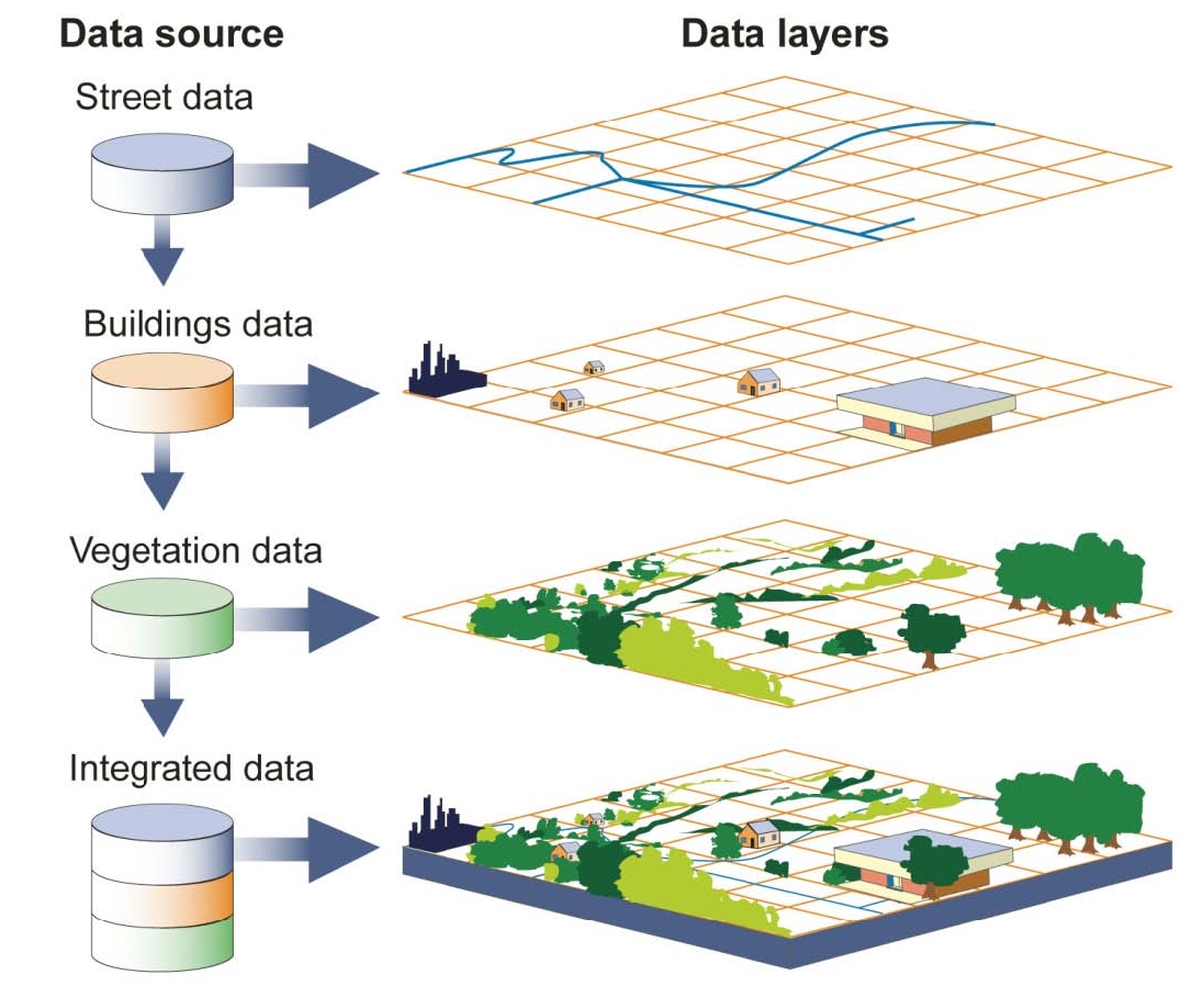
So let’s agree a scalar field can be described as an object. What happens when we have several scalar fields that describe the same space? Lets consider a real world example. There is a landscape. There are a set of quantities that vary over the landscape, like elevation, rain, or height. How do you go about representing the landscape in an object oriented fashion? Do you create a “rock column” class to aggregate the quantities at a particular point? If so, then you never implement the scalar field class. Obviously, object oriented design can be achieved in many ways, and it is up to us to decide which design suits our needs.
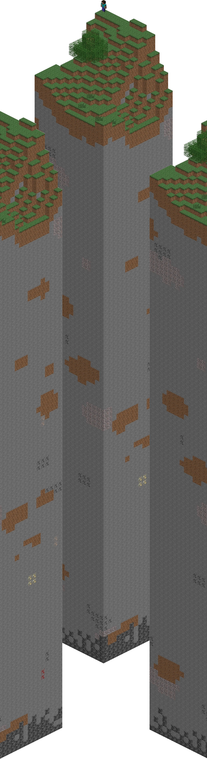
So which design suits our needs? Does the landscape grow or shrink, like with chunks in Minecraft? In that case, AoS is clearly the best option. But what if the landscape is static? What if you work on GIS software, and the quantities you track all come from many data sources that each work with different resolutions?
 |
 |
|---|---|
| AoS | SoA |
Clearly, there is some reason to use SoA in OOP, and as we’ll see, SoA fits in nicely with the math we use.
The Math
We mentioned the Navier Stokes equation as a way to mathmatically describe the motion of fluids. But what is it?
`(delv)/(delt) + (v*nabla)v = -1/rho nabla p -nabla phi + 1/rho eta nabla^2 v + (eta + eta') nabla(nabla*v)`
At it’s core, it’s really just a restatement of newton’s second law
`F = ma`
Force is mass times acceleration. If you want to know how much a parcel of fluid changes its velocity, then you rephrase it as:
`a = 1/m F`
In our model, we’re dealing with parcels of fluid with constant volume, so we express mass in terms of density
`a = 1/rho F`
where `rho` is density. Now all you need is to describe your forces on the right hand side. The equation accomodates forces like gravity, viscosity, and pressure, but we won't describe all these things. Lets just take pressure as an example:
`a = -1/rho nabla p`
What's this triangle character, `nabla`? Oh, that's nabla. It's a vector representing the amount of change across each cartesian coordinate (in this case, x,y, and z). `nabla p` is the change in pressure across each of the cartesian coordinates. We call it the pressure gradient. The pressure gradient looks like a vector that points in the direction of greatest pressure increase. So that means `-nabla p` points in the direction of greatest pressure decrease. Ever heard how fluids move from high pressure to low pressure? Well this is the mathematical restatement of that.
`nabla` is a vector, and just like any other vector you can apply the dot product to it. This dot product is the cumulative change in a vector's components across all cartesian coordinates. We call it the divergence because a positive value indicates an area where vectors point away from one another. For a vector v the divergence is written `nabla * v`. `nabla * nabla p` then is the cumulative change in pressure gradient across all cartesian coordinates. We call it the pressure Laplacian (after a man named Laplace). If there's a sudden low pressure region across a field, the pressure gradient suddenly points away from it. The components of the pressure gradient vector move from positive to negative, so `nabla * nabla p` takes on a negative value. The negation, `-nabla * nabla p`, is positive for low pressure regions and negative for high pressure regions, and this perfectly describes the change in pressure over time (`(del p) / (del t)`) as fluid fills in low pressure regions and drains from high pressure regions. So we write:
`(del p) / (del t) prop -nabla*nabla p`
This is the equation that Tectonics.js currently uses. It resembles a very well known equation. It appears all the time in physics, and it even has its own name: the diffusion equation.
Tectonics.js uses this equation to approximate the 2d motion of the mantle, as we’ll see below.
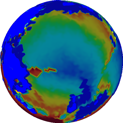
The Implementation
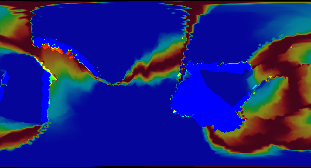
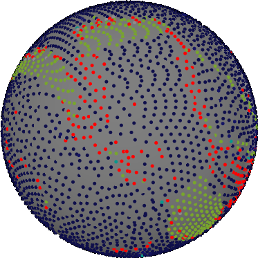
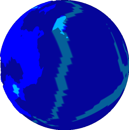
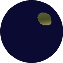
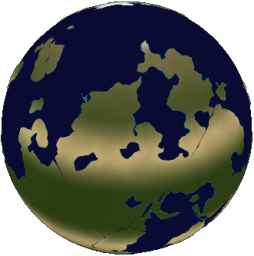
It starts off with crust age (older crust is blue):
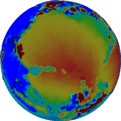
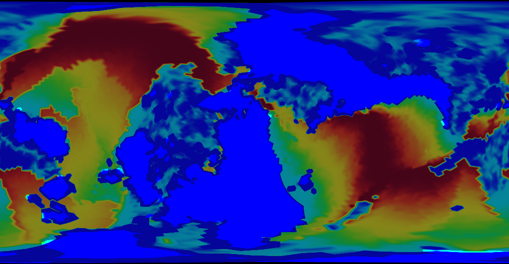
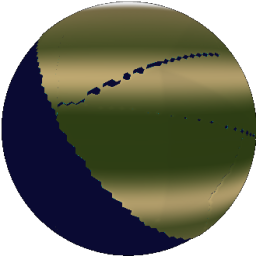
Age is used to calculate density. Oceanic crust gets dense (red) with age:
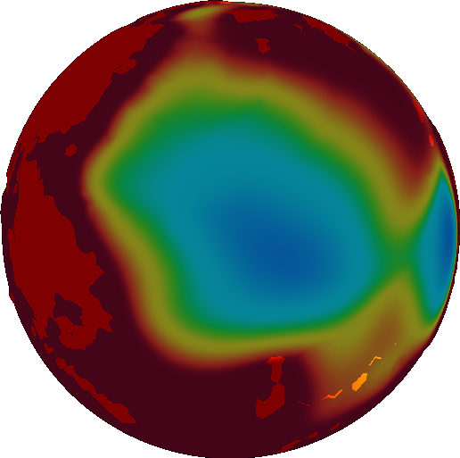
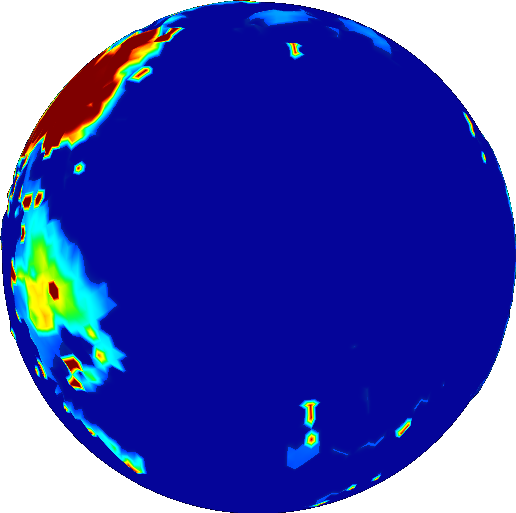
If density get above a certain threshold, the crust founders (shown in blue):

We still have a ways to go before we find the velocity. We could take the gradient for foundering, but it doesn’t represent velocity well. All the arrows are confined to the transition zones between foundering and non-foundering.
We want our velocity field to be fairly uniform across a single plate. So we smooth it out using the diffusion equation, mentioned above.
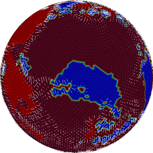
Now we’re ready to take the gradient to find velocity.
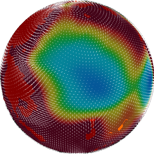
Now velocity is somewhat heterogeneous, and this won’t do for us. We want to treat our plates as rigid bodies, with constant velocity throughout. Doing so requires us first to define where these plates exist. In real life, the solution probably lies in fracture mechanics, but Tectonics.js takes a different route. It runs an image segmentation algorithm over the angular velocity field. This breaks up the velocity field into regions with similar velocity. The image segmentation algorithm needs a metric to compare velocity to determine whether two grid cells belong in the same segment. This has an obvious solution for scalar values, but it’s a little less obvious when working with vectors. No matter - image segmentation algorithms are run every day on color images, and color images are nothing more than vector fields. Just as is done with color images, we use cosine similarity to determine the similarity between vectors.
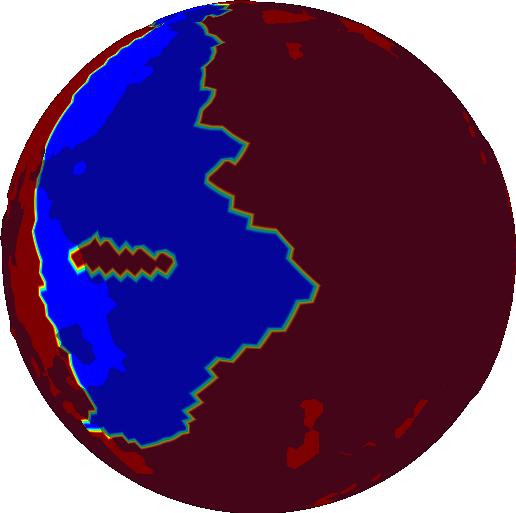
The image segmentation algorithm we’re currently using works by repeatedly performing the Flood Fill algorithm. Every iteration, the image segmentation algorithm finds the largest uncategorized vector in the field, then fits it into a new category using the flood fill algorithm. Binary morphology is used with every iteration to round out the borders.
The first iteration looks like this:
The last iteration looks like this:
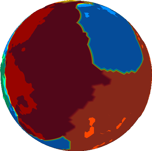
We now have a list of segments, each of which is represented by a bit mask. Find the average angular velocity field over the bit mask and we find the angular velocity of the plate. We can think of this as a weighted average of angular velocity across the field, where the weights are given by the bit mask.
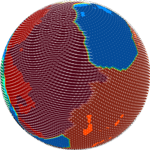
The rest is just what the model has always done: destroy crust at intersections, create new crust at gaps. But now we’re using rasters as objects, so we have a much more robust framework for expressing our intended behavior. We use binary morphology to identify where crust must be created or destroyed. There is a ready made “intersection” operation that identifies where crust must be destroyed
, and the negation of a union identifies where crust must be created. Because crust can only be created or destroyed at the boundaries of plates, we take either the dilation/erosion plate, and then perform the difference with the original plate to find the boundary. These aren’t standard operations in morphology, but they are so commonly used I created individual functions for them, called “margin” and “padding” in allusion to the html box model.
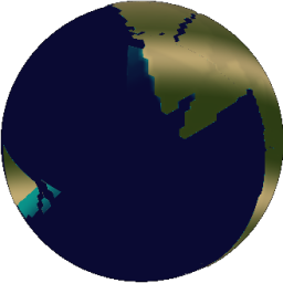
The results are promising.
Ah, much better. Oceanic crust is much younger now that our model deliberately destroys old crust. Go figure.
Architecture
We’ve made use of a few paradigms to get this point:
- We use vector calculus to find properties like asthenosphere velocity, which is the laplacian of a subductability metric.
- We use rasters to represent scalar fields within our code. Resampling is done to convert between rasters of different coordinate systems.
- We use image analysis to identify plates.
- We use statistics to identify the angular velocity of plates.
- We use binary morphology to identify regions where crust is created or destroyed.
These paradigms were historically derived in isolation. Concepts may be easy to understand in one paradigm, but unorthodox or even non-existant in another. The only commonality they share is that they are represented as rasters within our code.
If our code is to be flexible, it must allow us to experiment effortlessly with different paradigms and their combinations. We must be able to switch paradigms effortlessly, without any type conversion.
The solution I found is to build the project around a set of primitive “raster” data types, then handle operations on these data types over a series of namespaces. Each namespace corresponds to a paradigm.
Nothing about the raster data types will be encapsulated. The namespaces have free reign over the rasters. The primary function of the namespaces is to create a separation of concerns, and I am trading encapsulation in order to achieve that.
There are several raster data types, and they differ only in what type of data they store, e.g. Float32Raster, Uint8Raster, VectorRaster. The raster datatypes will be kept as primitive as possible: no methods, and very few attributes. In Tectonics.js, these raster data types are represented as typed arrays with only one additional attribute, “grid”, which maps each cell in the typed array to a cell within a grid. The grid can be any arbitrary 3d mesh, but in practice Tectonics.js only uses them with spheroids with roughly equidistant vertices.
Each namespace corresponds to a paradigm mentioned above. Functions within a namespace are built for efficiency. The vast majority of runtime will be spent within these functions, so every piddling performance gain will be put to use in them. To this end, the method signatures all follow a similar format:
Namespace.function(input1, input2, output, scratch)
This method signature is designed to maximize performance and versatility. “output” is an optional raster datatype, and if provided, the function stores results in the raster provided, in addition to returning the raster in the normal way. “output” can be set to the same raster as “input1” or “input2”, in which case the function performs its operation in-place. “scratch” is another optional raster datatype provided in the event the function needs to store something in a temporary variable. Typed arrays can be very performant in Javascript, but they will kill performance if you create hundreds of them every frame, so the scratch parameter is a solution to that limitation.
Outside the functions, less attention is paid to performance. Most of the calling code is used infrequently by comparison (maybe once or twice per frame), and the raster functions hide away the optimizations. This allows us a good balance of readability and performance.
The same sort of call structure can be extended to other parts of the model. We can construct functions that are similar to the ones above in order to perform operations within the model. For instance, here’s the function we use to calculate erosion:
TectonicsModel.get_erosion = function (
        displacement, sealevel, timestep, // input
        erosion,                          // output
        scratch1, scratch2                // temp storage
){
  erosion               = erosion  || Float32Raster(displacement.grid);
  var water_height      = scratch1 || Float32Raster(displacement.grid);
  var height_difference = scratch2 || Float32Raster(displacement.grid);
  var rate = ... // some constant
  ScalarField.max_scalar (displacement, sealevel,               water_height);
  ScalarField.laplacian  (water_height,                    height_difference);
  ScalarField.mult_scalar(height_difference, timestep * rate, erosion);

  return erosion;
}
A planet’s crust is nothing more than a tuple of rasters. We can create a “Crust” class composed of several rasters, then construct a set of functions that use the same kind of method signature to perform larger operations. For instance, here’s the function used to copy Crust objects:
Crust.copy = function(source, destination) {
  Float32Raster.copy(source.thickness,   destination.thickness);
  Float32Raster.copy(source.density,     destination.density);
  Float32Raster.copy(source.age,         destination.age);
}
One last thing. Now that we use a common data structure to express operations within the model, we can easily create a developer tool that consumes this data structure and visualizes it. Pass it any callback function that generates a field, and the field will be displayed on screen.
We’ve already seen how this can be used.
This turned out to be really easy to implement. Version 1.0 of the model already had a “View” class as part of the MVC pattern. All that was needed was to modify the View class to include the aforementioned callback function as an attribute, then pass it to the 3d graphics library. The callback function is called once per frame, so the visualization can update in real time.
I can’t overemphasize the importance of visualization. I’ve watched presentations at game developer conferences and it often seems they only brag about the developer tools they built, but now I understand why. Visualization radically improves the turn around time for model development.
Let’s say you found a bug with the erosion model (shown previously). Back in Version 1.0, you’d either have to examine its effects indirectly, or you’d have to spend a lot of time creating a new View subclass that you know you’d never use again. Now all I have to do is open up my browser’s JS console and type something like:
view.setScalarDisplay(
  new ScalarHeatDisplay(  {
    min: '0.', max: '10000.',
    getField: function (world) {
      return TectonicsModel.get_erosion(world.displacement, world.SEALEVEL, 1);
    }
}));
It gives me great hope for the future of the model.
The Moral of the Story
Object oriented programmers will have noticed something by now. My tectonics model revolves around these “objects” that are best described as Structures of Arrays with no methods and no encapsulation. Why even bother calling them “objects”?
Indeed.
If I’ve learned one thing from this experience, it’s to stand up for yourself and say “no” to best practice. Sometimes your perception of best practice is something completely different than what best practice actually is, and othertimes, best practice just does not apply. I spent a long time doing nothing because SoA didn’t jive with my preconceptions of OOP best practice, and I spent a long time doing nothing because encapsulation didn’t work with my raster namespacing. Best practice exists to achieve certain objectives that most people have. It does not exist to save you from thinking. Understand what best practice is trying to do, understand what you are trying to do, and see where they meet. Think for yourself.
Implications
It’s sometimes hard to remember: all this started when I noticed crust age was wrong. This all seems like a lot of work for such a small thing, but it stopped being about crust age a long time ago.
This wasn’t just a change meant to fix crust age. It was a correction to the way the model works on the most fundamental level, and it opens a wide path to future development. We now have a framework to express any operation on a world’s crust in a manner that is clear, concise, and performant. We have a general purpose library that seamlessly integrates raster operations across multiple disparate mathematical paradigms. We have a Visualization tool that makes it incredibly easy to visualize and experiment with rasters. And as long as this writeup has become, I still don’t think I can fully capture everything this overhaul has enabled.
Rock type, sedimentation, wind, ocean currents, realistic temperature. All these are well within reach.
Model initialization using a Fractal Algorithm
August, 21 2015
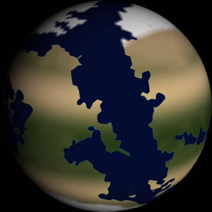
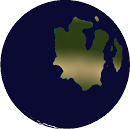
I’ve done some work to improve world initialization. Long time users will recall how the model always initialized with a single perfectly circular seed continent.
It now initializes worlds with continents of arbitrary shape. The world nevertheless maintains a hypsography similar to that of Earth.
How does it do this? With 2D models there are an abundance of algorithms used for generating terrain. There’s diamond square, perlin noise, brownian surfaces, genetic algorithms… None of these translate well to 3D, though, and there’s not a lot of algorithms that are tailor made for the circumstance. Really, I’ve only found one serious contender. This algorithm was first described by one Hugo Elias, then later improved upon by one Paul Bourke. Its original creator is unknown to me. The method is simple enough:
- divide the planet in half along some random axis
- add height to one of the halves
- repeat as needed
The more iterations, the better it looks.
 |
 |
|---|---|
| 1 iteration | 10 iterations |
I’ve made a few contributions to the algorithm in my attempt to adapt it to the model. I’ll describe these contributions later, but first I want to describe this algorithm mathematically.
Think about what happens in step 2, where you increase elevation depending on what side you’re on. Consider the simplest case where the “random axis” happens to be the planet’s axis of rotation. We’ll call this the z component of our position vector. Now, we want everything in the northern hemisphere to increase in height. In other words, we increase elevation where the z component is positive. We’ll use the Heaviside step function to describe this relation:
`Delta h prop H(x_z)`
Where `Delta h` is the change in height, and `vec(x)` is our position in space.
Now, back to step 1. We want to orient our northern hemisphere so that it faces some random direction. We can do this by applying a matrix to `vec(x)`. This matrix, denoted `bb A`, represents a random rotation in 3D space.
`Delta h prop H((bb A vec(x))_z)`
We only wind up using the z component of the matrix, so this simplifies to taking the dot product of a random unit vector, denoted `vec(a)`.
`Delta h prop H(vec(a) * vec(x))`
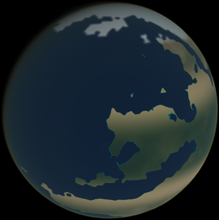
There are a few commonly cited problems with this algorithm. One problem occurs when you zoom in on the world. You start to see a bunch of straight lines that mark where the world was divided.
You can mask this by increasing the number of iterations, but it still looks jagged - almost as if the world has no erosion.
 |
 |
|---|---|
| 50 iterations | 500 iterations |
This problem has a rather obvious solution - use a smoother function. In my model, I use the logistic function, which is commonly used as a smooth approximation to the Heaviside:
`H(x) ~~ 1 / (1 + e^(-2kx))`
A larger value for k corresponds to a sharper transition. For my model, I set `k ~~ 300`. This is suitable for use with a unit sphere where `-1 < x_z < 1`.
 |
 |
|---|---|
| k = 50 | k = 300 |
Another problem with the algorithm concerns the realism of the heights generated. Paul Bourke aluded to this when he noted that a planet generated this way would be symmetrical. Oceans on one side would perfectly match the shape of continents on the other side.
Paul's solution was to offset `vec(a) * vec(x)` in the equations above by some random amount. The effect of this was to make one of the hemispheres slightly larger than the other.
`Delta h prop H(vec(a) * vec(x) + b)`
However, the problems run deeper than this. Earth follows a very specific hypsographic curve. The curve is bimodal - oceans cover 71% percent of earth, with the remainder taken up by continents. There is a very sharp transition between oceanic and continental crust, and this transition is known as continental margin. Outliers like mountains or trenches occur rarely. We need to encompass all these facts in our algorithm. Moreover, we don’t want a solution that just looks good. We want a solution that exactly matches this hypsography.
There’s no way we’re going to accomplish this by tweaking the existing model parameters. The solution requires us to use Earth’s hypsographic curve as its own model parameter.
The hypsographic curve is a probability density function that tells us the probability of finding a piece of land with a given elevation. We can use this probability density function to generate a series of random values. These random values will serve as the elevations that populate our world. On earth, hypsography can be represented by the following statistical model:
`h ~ {(N(-4019, 1113), if f_{ocean} > 0.71), (N(797,1169), if f_{ocean} < 0.71):}`
`f_{ocean} ~ uni f(0,1)`
where `h` is height in meters, and `f_{ocean}` is a means to express the fraction of earth covered by ocean. `N` and `uni f` are the normal and uniform distribution functions, respectively.
But how do we map these elevations to location? That's the job for our algorithm. Our algorithm may not be able to provide us with elevation, but it can tell us which areas need to be high or low. For each grid cell in the model, our algorithm could be said to generate a height rank, `h_r` such that:
`Delta h_r = H(vec(a) * vec(x))`
Where `Delta h_r` is the change in height rank with each iteration of the algorithm.
If we sort our grid cells by height rank, we get a sense for which cells are high or low. All that’s left is to sort a randomly generated list of elevations and pair them up with our ordered list of grid cells. Each grid cell now has an elevation that is in keeping with the hypsographic curve.
The technique is remarkably flexible. I can generate a planet similar to Earth, or Mars, or any other planet for which the hypsographic curve is known. I can also decompose Earth’s hypsographic curve, seperating curves for ocean and land. I can combine these curves in any ratio to produce a planet with a specific percentage of ocean cover.
The technique is also easily abstracted. It’s apparent the method works equally well for any terrain generation algorithm, but it goes beyond that. It can work for any procedural algorithm that describes a scalar field, and it works particularly well when that procedural algorithm can’t reproduce a probability distribution found in nature.
Now, there is still one lingering problem. The algorithm we’ve discussed works well for generating realistic elevations. However, our tectonics model needs this expressed in terms of crust density and thickness. The solution is to interpolate these parameters from a series of control points. So far the model uses simple linear interpolation, so for each grid cell we find the two control points whose elevation most closely matches our grid cell, then interpolate between their values for density and thickness.
| Control Point | Elevation (m) | Thickness (m) | Density (kg/m^3) |
|---|---|---|---|
| Abyss | -11000 | 3000 | 3000 |
| Deep Ocean | -6000 | 6300 | 3000 |
| Shallow Ocean | -3680 | 7900 | 2890 |
| Continental Shelf | -200 | 17000 | 2700 |
| Land | 840 | 36900 | 2700 |
| Mountain | 8848 | 70000 | 2700 |
Saves and Exports
May, 17 2015
There’s been a few recent items in the project’s issue tracker. They’d been slowly accumulating while I was busy focused on other projects. I decided to get back to the project to implement some much needed functionality.
First on the chopping block: implement some way to export a world to a format that’s readily consumable as a texture in a 3d model file. For a while now, the application’s been able to do this to some capacity through screenshots. Screenshots are a good starting point, but outstanding issues with the display made it arduous to convert from screenshot to texture file.
Circumstances involving the implementation of the equirectangular projection meant edges of the map were jagged. These jagged edges loosely corresponded to vertices in the icosahedrons used to represent tectonic plates. To resolve this issue, a second mesh is generated for each plate represented by the simulation. This second mesh differs only by an offset that’s used to express which side of the screen it should render on. This modification really highlighted the benefit of using a model/view based architecture - meshes used to represent the plate were kept seperate from the meshes that were actually rendered to the screen, so adding an duplicate mesh for the render didn’t have to mean duplicating properties of the model.
There was also a need to generate equirectangular maps in a manner that was able to occupy the whole screen. This was to prevent the user from having to manually crop screenshots in order to make a texture. This was easy enough and amounted to a few lines of shader code.
Textures aren’t even the limit to what could be done as far as exporting goes. It’s planned at some point to export the entire 3d model, textures and all. I don’t see too many things holding this back. The mesh itself is just a sphere - it can be kept as a static file on the server. I expect the bulk of the work will be in packaging this with the texture and sending it off to the user. With textures out of the way, though, exporting meshes assumes a lower priority in comparison to other items in the issue tracker.
Speaking of which, there was another item in the issue tracker for implementing some means of saving and retrieving model state. The actual ideal is to store the model state in the url itself, allowing a permalink to be generated for any arbitrary world. This link could then be shared effortlessly over the internet, without need for things like file hosting.
From what I calculate, this is going to be an unrealistic vision. A single model run uses somewhere around 10,000 grid cells, each with at least 8 bytes of floating point data. I’m firm on this number - I won’t accept any loss of resolution on account of the save feature. A naive implementation would take 80KB to store the model, at best. By using 2 byte floats, you could reduce this number to 40KB, which is far higher than the 8KB allowed in the address bars of most modern browsers. This says nothing of any future changes I’ll want to make to model state, some of which could grossly inflate the size of save files.
Still, that’s not stopping me from doing something I’d already planned to do with model: file saves. File saves are a necessary intermediary if ever it does turn out to be possible to encode model state in a url. One way or another, the model has to be reduced to a form that can be expressed acyclically without functions or other complex data structures. Once you have that, its relatively easy to encode it in a string and save it to a file.
Current file size is pretty consistently 170KB. As mentioned, I’m reasonably confident this number can go down to 40KB. I’m doubtful whether compression would be able to bring this into the range needed to use a query string parameter, though
At present, the save file format offers no guarantees on forward compatibility. Don’t get too attached to the worlds you save.
Reddit and erosion
January, 29 2014
So, what do these two things have in common?
Last Saturday I debuted the simulation to the fine folk of the /r/worldbuilding subreddit. Its a small community dedicated to the creation of sci fi and fantasy worlds with a strong emphasis on mapmaking. I’ve posted there a few times, generally demonstrating a toy world I modeled by hand. This was actually the project that lead up to the creation of PyTectonics, the predecessor to the simulation you see here.
The feedback there was very informative. I was surprised to see interest in some things I’d previously thought the public wouldn’t pay much attention to in a model - sea floor height, for instance. Other suggestions, on the other hand, I knew would be brought up at some point - the comments made very clear the need for realistic mountains. While the model at the time still technically simulated mountains, the lack of an erosion model was presumably causing them to get out of hand, eventually occupying every available cell of continental crust. An erosion model would be needed before mountains could be integrated into the main satellite view.
Fortunately, I’ve had a solid erosion model lined up for some time, now. What’s beautiful about this model is its ability to simulate erosion over large space and time scales, such as those you’d expect from a plate tectonics simulator. I’d seen many published erosion models while researching the problem, but almost all of them dealt with the spatial scales and timespans you’d need to, say, model the formation of a river system.
Don’t let the dense prose fool you - the model is stupid simple at its core. For each pair of neighboring grid cells, the model takes the height difference between the two and transfers a fraction of that height from one cell to another. The fraction that gets transferred is determined by two parameters:
1.) precipitation
2.) rate of erosion, expressed as a fraction of height per unit of precipitation
That’s it. The original publication embellishes upon this to partition bedrock erosion from sediment erosion, and I might do something like this in the future, but for now the model works good enough. Precipitation is also currently set to a constant reflecting the average rainfall experienced on Earth, but again, good enough.
So mountains are less frequent, now. There are still issues though:
1.) Mountains are still much taller than those encountered on earth, say, 15km.
2.) Coasts occassionally appear much more rounded than what we see on earth.
Both may be symptoms for a number of problems that are both hard to pin down. It may be that the erosion parameters require calibration, but any parameter changes made to address one issue will likely exacerbate the other. Setting precipitation to something besides a constant may be a more plausible solution. Coasts may not be as well rounded if they reflect gradients in precipitation, doubly so if certain regions receive hardly any precipitation, whatsoever. Mountain height might still be overpredicted, but at least then calibration could be conducted on it without exacerbating issues with the coastline. Issues with mountain height may also be addressed by calibrating parameters that define the rate at which continental crust accretes. Previously I was wary to touch these parameters since the model was already predicting a reasonable landmass percentage, but landmass appears to have increased in size now that there is erosion, and it might be time to reinvestigate the accretion parameters.
New Youtube Video, and a New Release
January, 25 2014
A new Youtube video is uploaded. You can check it out here:
The new video is intended to demo the app for users who lack the required support for WebGL. The video also demos features for a new release to the model. Perhaps most noticeable, the application’s graphic shader now displays a number of additional biomes, including jungle, desert, taiga, and tundra. As with previous versions, colors for each biome are sampled from real satellite imagery. The method used to determine biomes is a simple function of latitude - you’d probably scoff if you saw the code. I largely intended to portray to world builders a first order approximation at where they could expect to find certain biomes in their world. The world builder can go from there, if so inclined. Considering the small amount of time that went into implementing this feature, I’m still very pleased with the result.
The second feature that comes with this update allows the user to view his world from a number of views and projections. This was something that had bogged down the development of the project’s predecessor, pyTectonics, however with this iteration the feature was implemented very painlessly with the extensive use of 3d shaders. The roles of views and projections are so well partitioned among fragment and vertex shaders that no additional code had to be written outside of glsl - events for projection and view controls map directly to a corresponding vertex and fragment shader. So far only two options exist for each shader type, but I expectt this will change as need arises.
A Message to IE users
January, 19 2014
Recently I’ve been building up the web site to better handle cases in which the simulator simply cannot run: cases in which javascript is disabled, for instance, or cases in which the browser does not enable webgl by default. One of the more noteworthy cases are those in which the user is trying to view the simulator from an older browser that does not support WebGL, and thanks to the transformative adoption of Evergreen browsers this case almost exclusively applies to old man Internet Explorer.
To be fair, IE10 and above both appear to run simulations with acceptable performance. This will continue for as long as I care to use the technologies that they support, but I’m not really going to take it into consideration the next time I see a useful new web technology. Adoption rates for IE6 and 7 also thankfully no longer require consideration. China is exceptional, but they can go add me to their blacklist before I’ll try supporting IE6. In any case, this post does not apply to these versions. Thanks to a combination of user negligence and developer incompetence, IE8 and IE9 still holds a legitimate portion of the browser market. This fraction will reduce with time, but the case still needs to be considered. Rather than cripple the simulation, I figure: why not have some fun with it?
Tectonics, now in your browser!
December, 1 2013
After perhaps a month or two of incubation, a proper project website has emerged for the tectonics.js simulator. Updates will be posted to this website from time to time documenting progress on the model in addition to the accounts of technologies, problems, and solutions encountered in the project’s development.
This project comes as the successor to an earlier plate tectonics simulator, PyTectonics. Like Tectonics.js, this project set out to create a 3d tectonics simulator. Unlike Tectonics.js, it did so using the Python programming language, and as such the projects have differing ideals concerning readability and audience. Taking the Pythonic approach, PyTectonics set out to err on the side of readability at the expense of performance. Given the nature of its subject matter and emphasis on readability, the simulation was largely targeted towards likeminded developers.
Tectonics.js is the culmination of lessons learned over the course of developing the earlier pyTectonics program. Chief among these lessons I believe was learning the need for a wider audience in a project of this nature, and in turn the need for technologies that minimize the knowledge required from the user. The niche for a simulator such as tectonics.js is admitantly small and often those who are interested in the project are not necessarily those capable of participating in its development. A person doesn’t need to know how a model works in order to appreciate its output or base his work of fiction on it. All he needs is assurance the model will produce results in accordance with what geologists generally think happens in reality.
With web apps this is largely a nonissue. Any user can click a link. Being asked to use a different browser is a much different experience from being asked to install python and a list of libraries. Any libraries you need can be imported with impunity, and I use this advantage with extreme prejudice - already the simulation is working with underscore.js, as well as libraries implementing kd trees, data structures, and random number generators.
This last point leads into a second lesson emphasizing the importance of mature libraries with a large userbase. Without criticizing Python’s 3d libraries, the web is rapidly converging on technologies used for developing 3d applications, most notably the WebGL API and the three.js library that the new project has come to depend on. The large community that surrounds these technologies in turn often reduces the effort required in finding your own solutions to problems.
Another lesson learned concerns efficiency. PyTectonics started under the assumption that a lot changed since the days of SimEarth, the project’s spiritual predecessor. A new simulator could make no compromise on readability and still deliver adequate performance for the user, if only through concentrating on the efficiency of algorithms. This turns out to be only partially true. PyTectonics as it currently stands delivers arguably adequate performance and code remains pythonic. Oftentimes, the most readable solution has turned out to double as the most efficient solution, as well. However, a problem arises when one considers the algorithmic shenanigans going on in order for python to perform adequately. A good example of this is in detecting plate borders so that collision detection can occur efficiently - a single list is created for each plate on initialization and that list is added to or detracted from whenever the plate changes shape. Every individual line of code is fairly readable in the process, but collectively the model is convoluted by a lot of functions that don’t do much of anything besides saving runtime. I’ve come to the conclusion this ultimately hinders understanding. What’s more, the increased mental overhead makes it increasingly difficult to debug and build upon.
The move to pure javascript for the sake of efficiency sounds counterintuitive. It’s not. As it turns out, javascript on some modern web browsers is around five times faster than python. Here’s a figure reproduced from the study:
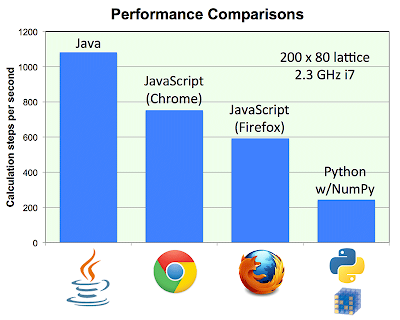
These tests were conducted on intense matrix operations, something very similar to what pyTectonics and company have to deal with. Even Safari offers speed comparable to python, according to these same tests. Based upon what’s been implemented so far in javascript, I’d have to agree. At the moment, my private development branch has loosely implemented both rifting and collision in javascript. These two operations from my experience in Python have taken up the majority of runtime. The time it takes to complete these operations varies strongly with the number of grid cells simulated by the application. At approximately 6000 grid cells, my python implementation maybe updates once every second. Threading is what prevents this implementation from becoming unresponsive to user input. Compare this to the javascript implementation, running in Chrome on the same machine - I can run around 10,000 grid cells in a simulation and still get a framerate of 20 fps, no threading whatsoever. I haven’t even considered the savings made once threading is taken into consideration, but rest assured that feature will come at some point.
Certain workarounds I mentioned before, such as caching plate borders, have still not been implemented. I really don’t care to do so. On the other hand, I’ve noticed things while re-implementing that could be done to improve performance without adding complexity to the simulation. It helps to have a robust 3d library like three.js to back you up. A good example is when geometries are updated. PyTectonics represents landmass as convex hulls that were partly occluded by the oceans. If crust rose out from the water, you would removed the object and created a new object with geometry reflecting the change. This was done every frame. Switching out objects was the only operation permitted by VPython, but with three.js, I have the option to manipulate individual vertices. Every plate starts out as an icosahedron and I push out vertices based on whether or not they should be above or below the water. I don’t doubt some of the efficiency improvements may have come from this.
There is only one caveat: tectonics.js will have to be run in a modern browser. Internet explorer 6 doesn’t count. Later versions of internet explorer will only work by virtue of complying with W3C standards. If there are any issues with even the most recent version of IE I won’t hesitate to drop support for it.
To see the simulator for yourself, just click here