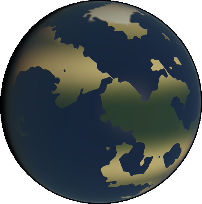
More than a year ago a feature request was filed on the Tectonics.js project repository. The request called for more visualizations within the model: crust age, mineral composition, and other cool features. This was something that I had wanted to implement for a long time. Crust age plays a big role in determining the density of oceanic crust, which in turn determines the motion of tectonic plates. Modeling crust age would be easy enough - simply add a new property to your rock column object and increment its value every update cycle. So I started with crust age. I setup the visualization and ran the simulation.
Then I saw the results.
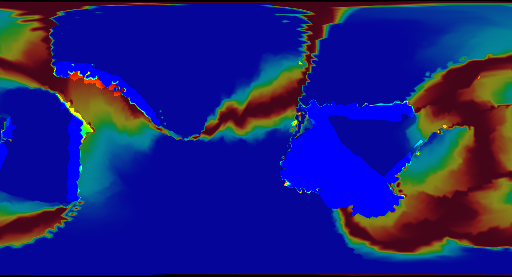
Ho boy. This wasn’t what I expected.
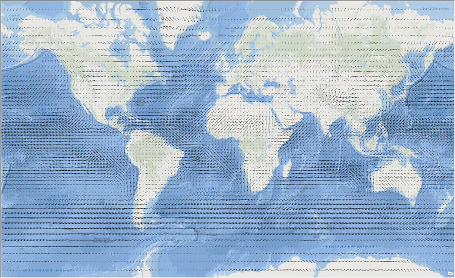
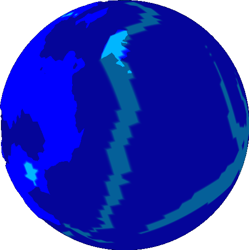
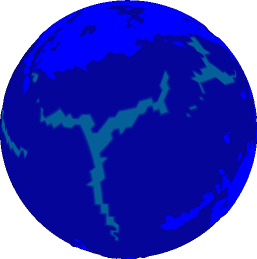
Take these results and compare them with Earth. The same colors are used to represent age.
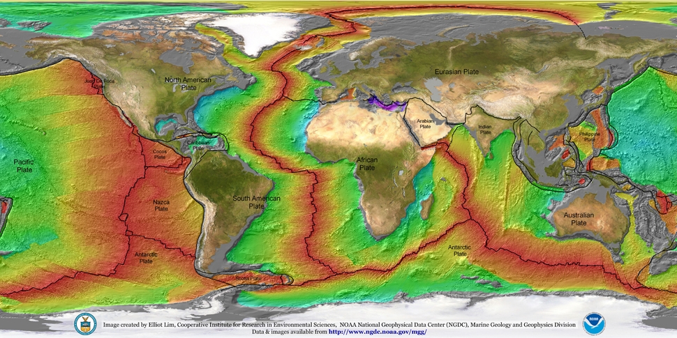
Notice anything different? The map of Earth is red. That means the ocean crust on Earth is much younger.
As a matter of fact, you’ll be hard pressed to find any ocean crust on Earth that’s older than 250 million years. This has to do with how the ocean crust responds to age. When ocean crust ages, it cools. When something cools, it becomes dense. When something becomes more dense than the liquid that surrounds it, it sinks. Sinking things drag down the other things they’re attached to. Things like tectonic plates. You can now start to see how this causes tectonic plates to move.
Now back to Tectonics.js. Look at virtually any simulation and you find ocean crust that’s well past this age, perhaps a billion years old or more. It isn’t too hard to find the reason. It comes down to what Tectonics.js was doing at its very core:
- generate a series of plates at random
- generate a series of velocities at random
- destroy crust whenever intersections occur
This is how its done in virtually every other non-academic tectonics simulator I’ve seen, and it’s wrong. There is simply no way you can reproduce Earth’s age distribution this way. Earth’s age distribution isn’t something you can reproduce by tweaking parameter values. The problem lies with the model itself.
I tried for a long time to solve the age problem with incremental change. Maybe you could keep your random plate geometry, but set the velocity to collide with nearby old crust? Maybe your plates could follow a predetermined path, one that maximizes their coverage of the globe? I spent several months trying these things off and on: considering them, designing them, implementing them, testing them. The experience left me deeply disheartened.
In an act of desperation, I took a new approach. Rather than start with the model and use it to produce the right output, I would start with the right output and then use it to produce the model.
An entire year passed as I redesigned the model from the ground up. I started the project as an experiment. I make a lot of experimental branches and most go nowhere. To outsiders, it probably looked like the project was abandoned, but truth is, I think this was one of the most productive years I’ve spent on the model.
The model that resulted was far removed from the original. Sure, the graphics look the same, but the internals were upended. Nothing was left untouched. I could only think of one way to describe it:
Version 2.0
Version 2.0 was such a change that I even debated creating a new website for it, but version 2.0 is so much better than the original that I don’t want to leave any uncertainty among the users:
Version 1.0 is a joke. Version 2.0 is the thing to use.
Only version 2.0 has an architecture that is flexible enough to implement all the things you ever dreamed of: atmospheric models, hydrological models, biosphere models, anything. Only version 2.0 uses the same mathematical framework that geophysicists use to model tectonics academically.
The Outset
I started out with one mantra, like a psychotic killer:
ocean crust must die.
If ocean crust is older than a certain threshold, it’s gone. No exceptions. Its like the Logan’s Run of oceanic crust. The model can keep old ocean crust in memory if it likes, but the pressure brought about by its sinking has to cause newer adjacent crust to take its place. Once it’s covered, it’s gone.
But how do you accomplish that? Well, nature does it somehow. So how does nature do it?
Over long periods of time, Earth’s crust behaves as a fluid, like a cup ouf cold pitch.
It seems like the perfectly correct answer involves some sort of fluid simulation. In case you’re wondering, no I don’t do fluid simulation. I don’t implement the Navier Stokes equation within the model. I just don’t have the computational power to do so. But I do use the same mathematical framwork. That framework is vector calculus. Its objects are scalar fields and vector fields.
What is a field? You already know what a field is. You see them in maps of elevation, temperature, and air currents, among other things. A field is a map where every point in space has a value. Sometimes, the value is a scalar, like temperature. Sometimes, the value is a vector, like air current.
For some time now, Tectonics.js has been able to display a number of fields: elevation, temperature, precipitation, plant productivity, etc. However, Tectonics.js never represented them as fields internally. Internally, Tectonics.js represented them in the canonical object-oriented fashion: a planet’s crust has an array of “rock column” objects, and each rock column object has a series of attributes for that specific point in space, like elevation or temperature.
function Crust() {
  this.rock_columns = [ new RockColumn(), new RockColumn(), ... ];
}

function RockColumn() {
  this.thickness = 0;
  this.density = 0;
  this.age = 0;
}
If you only wanted to see a single field, you would have to traverse the list of rock column objects and retreive the relevant attribute for each one. This sort of organization is known as the array of structures pattern, or AoS.
The alternative is known as a structure of arrays (or SoA). As a structure of arrays, a plate would store a series of attributes, each of which is an array of values corresponding to points in space. In other words, each attribute represents a field.
function Crust() {
  this.thickness = [0,0,0,...];
  this.density = [0,0,0,...];
  this.age = [0,0,0,...];
}
When I first developed Tectonics.js, I had a strong negative opinion of SoA. My day job at the time worked with R, and it exposed me to lots of situations where SoA was heavily abused.
A common example: let’s say we had a table represented by a structure of arrays.
function Table() {
  this.column1 = [0,0,0,...];
  this.column2 = [0,0,0,...];
  this.column3 = [0,0,0,...];
}
If the user wanted to insert or delete a column within a table, the same operation would be applied across all arrays within the structure. Now what happens when you want to add a row to the table? You have to go through every column and add the row at the correct index. Couple this with already badly written code and you have a nightmare on your hands.
Insertions and deletions were used to track associations between plates and rock columns. This was something done ever since the days of pyTectonics.
Each plate was represented as a grid populated by rock column objects, and when continental crust collides, rock columns were transfered from one plate’s grid to another. Under this regime the SoA pattern never seemed like the way to go.
However, my experience over time turned me away from the AoS approach. My time spent working on the model increasingly shifted towards solving collision detection, which was a slow and error prone process. Anyone who used the model previously may recall the patches of missing crust that occurred around collision zones, the planet-wide island arcs, or the massive continents that crumpled to narrow archipelagos from a single collision event.
What finally switched me over to SoA was the realization that AoS did not make sense from an object-oriented standpoint. I’m embarassed to admit it took an argument from OO to do so.
AoS always seemed like a very object oriented thing to do because it’s so natural to think of the “objects” as “structures” and not “arrays”. But what is an object? A mathematical vector could be an object, but why? Well, vectors have a set of operations, and these operations encapsulate attributes. But doesn’t the same apply to a scalar field? Why should mathemeticians abandon OOP if they want to use scalar fields?
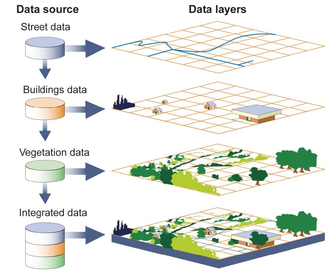
So let’s agree a scalar field can be described as an object. What happens when we have several scalar fields that describe the same space? Lets consider a real world example. There is a landscape. There are a set of quantities that vary over the landscape, like elevation, rain, or height. How do you go about representing the landscape in an object oriented fashion? Do you create a “rock column” class to aggregate the quantities at a particular point? If so, then you never implement the scalar field class. Obviously, object oriented design can be achieved in many ways, and it is up to us to decide which design suits our needs.
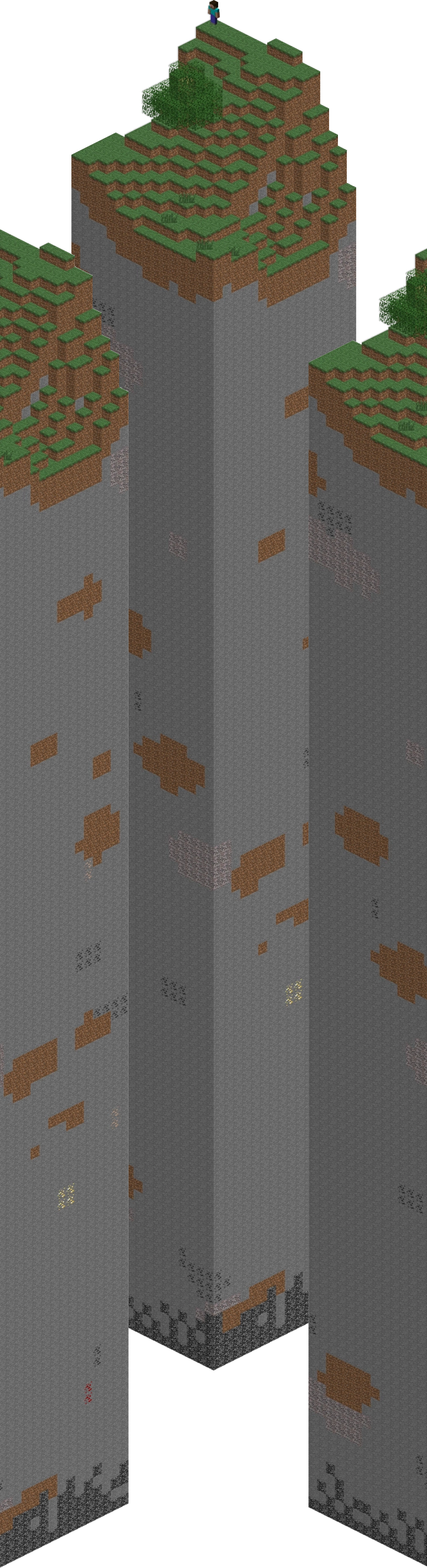
So which design suits our needs? Does the landscape grow or shrink, like with chunks in Minecraft? In that case, AoS is clearly the best option. But what if the landscape is static? What if you work on GIS software, and the quantities you track all come from many data sources that each work with different resolutions?
 |
 |
|---|---|
| AoS | SoA |
Clearly, there is some reason to use SoA in OOP, and as we’ll see, SoA fits in nicely with the math we use.
The Math
We mentioned the Navier Stokes equation as a way to mathmatically describe the motion of fluids. But what is it?
`(delv)/(delt) + (v*nabla)v = -1/rho nabla p -nabla phi + 1/rho eta nabla^2 v + (eta + eta') nabla(nabla*v)`
At it’s core, it’s really just a restatement of newton’s second law
`F = ma`
Force is mass times acceleration. If you want to know how much a parcel of fluid changes its velocity, then you rephrase it as:
`a = 1/m F`
In our model, we’re dealing with parcels of fluid with constant volume, so we express mass in terms of density
`a = 1/rho F`
where `rho` is density. Now all you need is to describe your forces on the right hand side. The equation accomodates forces like gravity, viscosity, and pressure, but we won't describe all these things. Lets just take pressure as an example:
`a = -1/rho nabla p`
What's this triangle character, `nabla`? Oh, that's nabla. It's a vector representing the amount of change across each cartesian coordinate (in this case, x,y, and z). `nabla p` is the change in pressure across each of the cartesian coordinates. We call it the pressure gradient. The pressure gradient looks like a vector that points in the direction of greatest pressure increase. So that means `-nabla p` points in the direction of greatest pressure decrease. Ever heard how fluids move from high pressure to low pressure? Well this is the mathematical restatement of that.
`nabla` is a vector, and just like any other vector you can apply the dot product to it. This dot product is the cumulative change in a vector's components across all cartesian coordinates. We call it the divergence because a positive value indicates an area where vectors point away from one another. For a vector v the divergence is written `nabla * v`. `nabla * nabla p` then is the cumulative change in pressure gradient across all cartesian coordinates. We call it the pressure Laplacian (after a man named Laplace). If there's a sudden low pressure region across a field, the pressure gradient suddenly points away from it. The components of the pressure gradient vector move from positive to negative, so `nabla * nabla p` takes on a negative value. The negation, `-nabla * nabla p`, is positive for low pressure regions and negative for high pressure regions, and this perfectly describes the change in pressure over time (`(del p) / (del t)`) as fluid fills in low pressure regions and drains from high pressure regions. So we write:
`(del p) / (del t) prop -nabla*nabla p`
This is the equation that Tectonics.js currently uses. It resembles a very well known equation. It appears all the time in physics, and it even has its own name: the diffusion equation.
Tectonics.js uses this equation to approximate the 2d motion of the mantle, as we’ll see below.
The Implementation
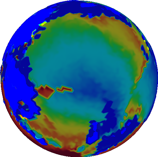
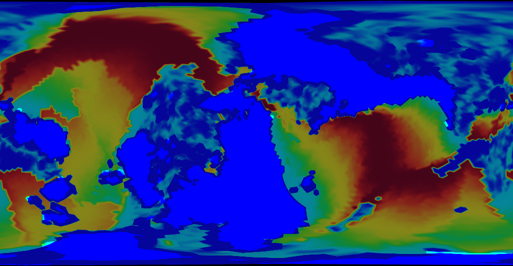
It starts off with crust age (older crust is blue):
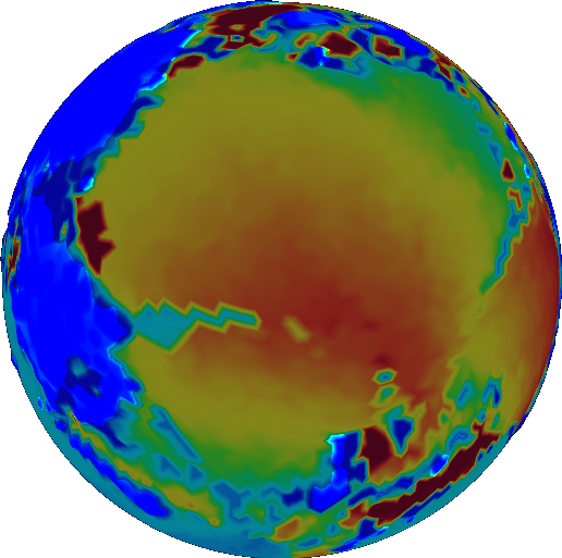
Age is used to calculate density. Oceanic crust gets dense (red) with age:
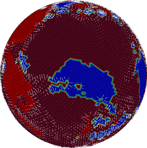
If density get above a certain threshold, the crust founders (shown in blue):

We still have a ways to go before we find the velocity. We could take the gradient for foundering, but it doesn’t represent velocity well. All the arrows are confined to the transition zones between foundering and non-foundering.
We want our velocity field to be fairly uniform across a single plate. So we smooth it out using the diffusion equation, mentioned above.
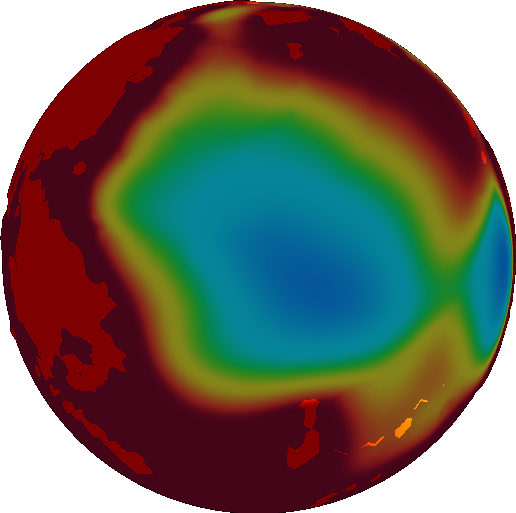
Now we’re ready to take the gradient to find velocity.
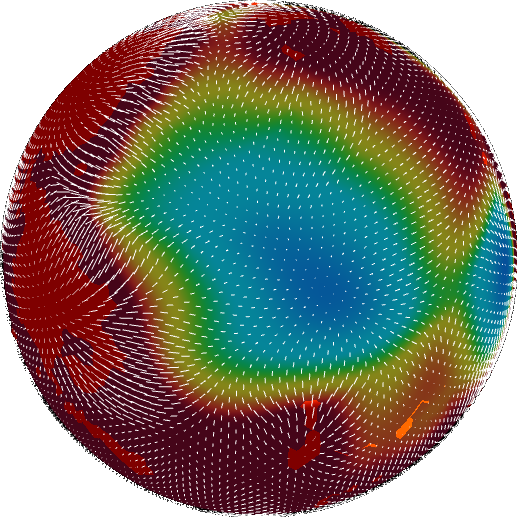
Now velocity is somewhat heterogeneous, and this won’t do for us. We want to treat our plates as rigid bodies, with constant velocity throughout. Doing so requires us first to define where these plates exist. In real life, the solution probably lies in fracture mechanics, but Tectonics.js takes a different route. It runs an image segmentation algorithm over the angular velocity field. This breaks up the velocity field into regions with similar velocity. The image segmentation algorithm needs a metric to compare velocity to determine whether two grid cells belong in the same segment. This has an obvious solution for scalar values, but it’s a little less obvious when working with vectors. No matter - image segmentation algorithms are run every day on color images, and color images are nothing more than vector fields. Just as is done with color images, we use cosine similarity to determine the similarity between vectors.
The image segmentation algorithm we’re currently using works by repeatedly performing the Flood Fill algorithm. Every iteration, the image segmentation algorithm finds the largest uncategorized vector in the field, then fits it into a new category using the flood fill algorithm. Binary morphology is used with every iteration to round out the borders.
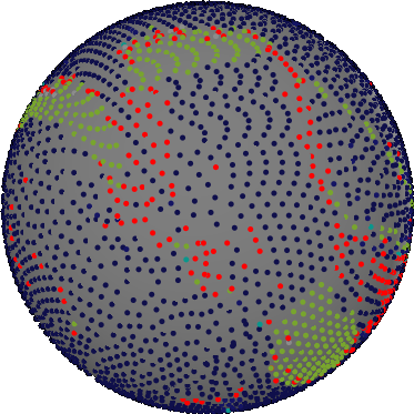
The first iteration looks like this:
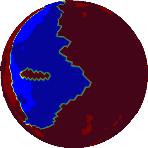
The last iteration looks like this:
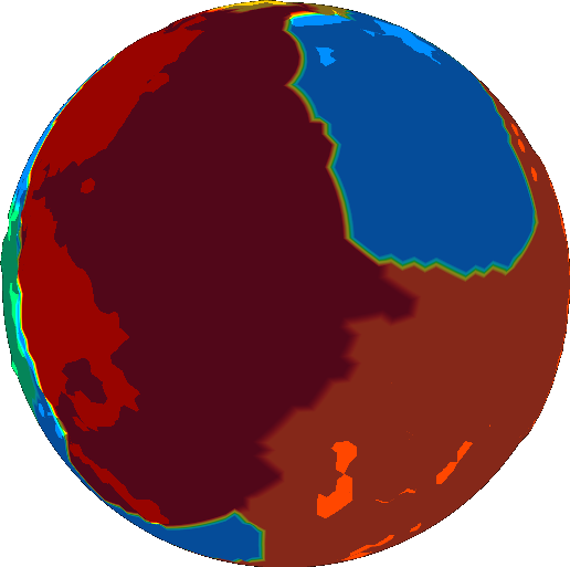
We now have a list of segments, each of which is represented by a bit mask. Find the average angular velocity field over the bit mask and we find the angular velocity of the plate. We can think of this as a weighted average of angular velocity across the field, where the weights are given by the bit mask.
The rest is just what the model has always done: destroy crust at intersections, create new crust at gaps. But now we’re using rasters as objects, so we have a much more robust framework for expressing our intended behavior. We use binary morphology to identify where crust must be created or destroyed. There is a ready made “intersection” operation that identifies where crust must be destroyed
, and the negation of a union identifies where crust must be created. Because crust can only be created or destroyed at the boundaries of plates, we take either the dilation/erosion plate, and then perform the difference with the original plate to find the boundary. These aren’t standard operations in morphology, but they are so commonly used I created individual functions for them, called “margin” and “padding” in allusion to the html box model.
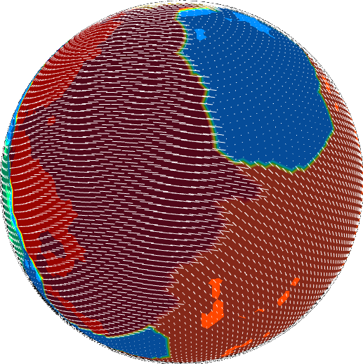
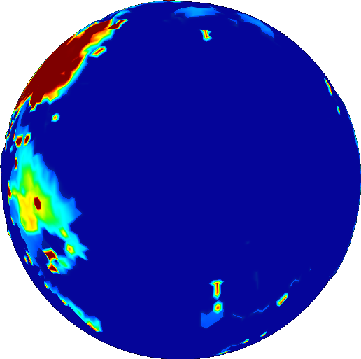
The results are promising.
Ah, much better. Oceanic crust is much younger now that our model deliberately destroys old crust. Go figure.
Architecture
We’ve made use of a few paradigms to get this point:
- We use vector calculus to find properties like asthenosphere velocity, which is the laplacian of a subductability metric.
- We use rasters to represent scalar fields within our code. Resampling is done to convert between rasters of different coordinate systems.
- We use image analysis to identify plates.
- We use statistics to identify the angular velocity of plates.
- We use binary morphology to identify regions where crust is created or destroyed.
These paradigms were historically derived in isolation. Concepts may be easy to understand in one paradigm, but unorthodox or even non-existant in another. The only commonality they share is that they are represented as rasters within our code.
If our code is to be flexible, it must allow us to experiment effortlessly with different paradigms and their combinations. We must be able to switch paradigms effortlessly, without any type conversion.
The solution I found is to build the project around a set of primitive “raster” data types, then handle operations on these data types over a series of namespaces. Each namespace corresponds to a paradigm.
Nothing about the raster data types will be encapsulated. The namespaces have free reign over the rasters. The primary function of the namespaces is to create a separation of concerns, and I am trading encapsulation in order to achieve that.
There are several raster data types, and they differ only in what type of data they store, e.g. Float32Raster, Uint8Raster, VectorRaster. The raster datatypes will be kept as primitive as possible: no methods, and very few attributes. In Tectonics.js, these raster data types are represented as typed arrays with only one additional attribute, “grid”, which maps each cell in the typed array to a cell within a grid. The grid can be any arbitrary 3d mesh, but in practice Tectonics.js only uses them with spheroids with roughly equidistant vertices.
Each namespace corresponds to a paradigm mentioned above. Functions within a namespace are built for efficiency. The vast majority of runtime will be spent within these functions, so every piddling performance gain will be put to use in them. To this end, the method signatures all follow a similar format:
Namespace.function(input1, input2, output, scratch)
This method signature is designed to maximize performance and versatility. “output” is an optional raster datatype, and if provided, the function stores results in the raster provided, in addition to returning the raster in the normal way. “output” can be set to the same raster as “input1” or “input2”, in which case the function performs its operation in-place. “scratch” is another optional raster datatype provided in the event the function needs to store something in a temporary variable. Typed arrays can be very performant in Javascript, but they will kill performance if you create hundreds of them every frame, so the scratch parameter is a solution to that limitation.
Outside the functions, less attention is paid to performance. Most of the calling code is used infrequently by comparison (maybe once or twice per frame), and the raster functions hide away the optimizations. This allows us a good balance of readability and performance.
The same sort of call structure can be extended to other parts of the model. We can construct functions that are similar to the ones above in order to perform operations within the model. For instance, here’s the function we use to calculate erosion:
TectonicsModel.get_erosion = function (
        displacement, sealevel, timestep, // input
        erosion,                          // output
        scratch1, scratch2                // temp storage
){
  erosion               = erosion  || Float32Raster(displacement.grid);
  var water_height      = scratch1 || Float32Raster(displacement.grid);
  var height_difference = scratch2 || Float32Raster(displacement.grid);
  var rate = ... // some constant
  ScalarField.max_scalar (displacement, sealevel,               water_height);
  ScalarField.laplacian  (water_height,                    height_difference);
  ScalarField.mult_scalar(height_difference, timestep * rate, erosion);

  return erosion;
}
A planet’s crust is nothing more than a tuple of rasters. We can create a “Crust” class composed of several rasters, then construct a set of functions that use the same kind of method signature to perform larger operations. For instance, here’s the function used to copy Crust objects:
Crust.copy = function(source, destination) {
  Float32Raster.copy(source.thickness,   destination.thickness);
  Float32Raster.copy(source.density,     destination.density);
  Float32Raster.copy(source.age,         destination.age);
}
One last thing. Now that we use a common data structure to express operations within the model, we can easily create a developer tool that consumes this data structure and visualizes it. Pass it any callback function that generates a field, and the field will be displayed on screen.
We’ve already seen how this can be used.
This turned out to be really easy to implement. Version 1.0 of the model already had a “View” class as part of the MVC pattern. All that was needed was to modify the View class to include the aforementioned callback function as an attribute, then pass it to the 3d graphics library. The callback function is called once per frame, so the visualization can update in real time.
I can’t overemphasize the importance of visualization. I’ve watched presentations at game developer conferences and it often seems they only brag about the developer tools they built, but now I understand why. Visualization radically improves the turn around time for model development.
Let’s say you found a bug with the erosion model (shown previously). Back in Version 1.0, you’d either have to examine its effects indirectly, or you’d have to spend a lot of time creating a new View subclass that you know you’d never use again. Now all I have to do is open up my browser’s JS console and type something like:
view.setScalarDisplay(
  new ScalarHeatDisplay(  {
    min: '0.', max: '10000.',
    getField: function (world) {
      return TectonicsModel.get_erosion(world.displacement, world.SEALEVEL, 1);
    }
}));
It gives me great hope for the future of the model.
The Moral of the Story
Object oriented programmers will have noticed something by now. My tectonics model revolves around these “objects” that are best described as Structures of Arrays with no methods and no encapsulation. Why even bother calling them “objects”?
Indeed.
If I’ve learned one thing from this experience, it’s to stand up for yourself and say “no” to best practice. Sometimes your perception of best practice is something completely different than what best practice actually is, and othertimes, best practice just does not apply. I spent a long time doing nothing because SoA didn’t jive with my preconceptions of OOP best practice, and I spent a long time doing nothing because encapsulation didn’t work with my raster namespacing. Best practice exists to achieve certain objectives that most people have. It does not exist to save you from thinking. Understand what best practice is trying to do, understand what you are trying to do, and see where they meet. Think for yourself.
Implications
It’s sometimes hard to remember: all this started when I noticed crust age was wrong. This all seems like a lot of work for such a small thing, but it stopped being about crust age a long time ago.
This wasn’t just a change meant to fix crust age. It was a correction to the way the model works on the most fundamental level, and it opens a wide path to future development. We now have a framework to express any operation on a world’s crust in a manner that is clear, concise, and performant. We have a general purpose library that seamlessly integrates raster operations across multiple disparate mathematical paradigms. We have a Visualization tool that makes it incredibly easy to visualize and experiment with rasters. And as long as this writeup has become, I still don’t think I can fully capture everything this overhaul has enabled.
Rock type, sedimentation, wind, ocean currents, realistic temperature. All these are well within reach.