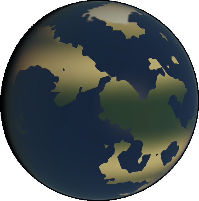
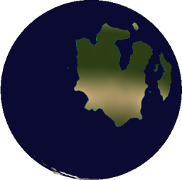
I’ve done some work to improve world initialization. Long time users will recall how the model always initialized with a single perfectly circular seed continent.
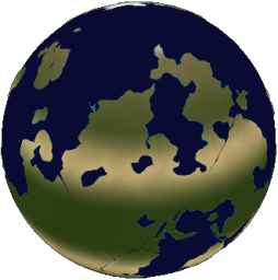
It now initializes worlds with continents of arbitrary shape. The world nevertheless maintains a hypsography similar to that of Earth.
How does it do this? With 2D models there are an abundance of algorithms used for generating terrain. There’s diamond square, perlin noise, brownian surfaces, genetic algorithms… None of these translate well to 3D, though, and there’s not a lot of algorithms that are tailor made for the circumstance. Really, I’ve only found one serious contender. This algorithm was first described by one Hugo Elias, then later improved upon by one Paul Bourke. Its original creator is unknown to me. The method is simple enough:
- divide the planet in half along some random axis
- add height to one of the halves
- repeat as needed
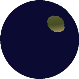
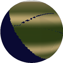
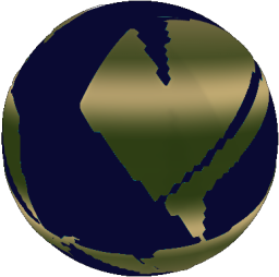
The more iterations, the better it looks.
 |
 |
|---|---|
| 1 iteration | 10 iterations |
I’ve made a few contributions to the algorithm in my attempt to adapt it to the model. I’ll describe these contributions later, but first I want to describe this algorithm mathematically.
Think about what happens in step 2, where you increase elevation depending on what side you’re on. Consider the simplest case where the “random axis” happens to be the planet’s axis of rotation. We’ll call this the z component of our position vector. Now, we want everything in the northern hemisphere to increase in height. In other words, we increase elevation where the z component is positive. We’ll use the Heaviside step function to describe this relation:
`Delta h prop H(x_z)`
Where `Delta h` is the change in height, and `vec(x)` is our position in space.
Now, back to step 1. We want to orient our northern hemisphere so that it faces some random direction. We can do this by applying a matrix to `vec(x)`. This matrix, denoted `bb A`, represents a random rotation in 3D space.
`Delta h prop H((bb A vec(x))_z)`
We only wind up using the z component of the matrix, so this simplifies to taking the dot product of a random unit vector, denoted `vec(a)`.
`Delta h prop H(vec(a) * vec(x))`
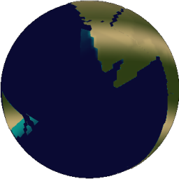
There are a few commonly cited problems with this algorithm. One problem occurs when you zoom in on the world. You start to see a bunch of straight lines that mark where the world was divided.
You can mask this by increasing the number of iterations, but it still looks jagged - almost as if the world has no erosion.
 |
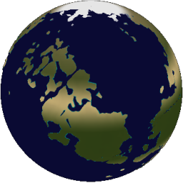 |
|---|---|
| 50 iterations | 500 iterations |
This problem has a rather obvious solution - use a smoother function. In my model, I use the logistic function, which is commonly used as a smooth approximation to the Heaviside:
`H(x) ~~ 1 / (1 + e^(-2kx))`
A larger value for k corresponds to a sharper transition. For my model, I set `k ~~ 300`. This is suitable for use with a unit sphere where `-1 < x_z < 1`.
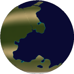 |
 |
|---|---|
| k = 50 | k = 300 |
Another problem with the algorithm concerns the realism of the heights generated. Paul Bourke aluded to this when he noted that a planet generated this way would be symmetrical. Oceans on one side would perfectly match the shape of continents on the other side.
Paul's solution was to offset `vec(a) * vec(x)` in the equations above by some random amount. The effect of this was to make one of the hemispheres slightly larger than the other.
`Delta h prop H(vec(a) * vec(x) + b)`
However, the problems run deeper than this. Earth follows a very specific hypsographic curve. The curve is bimodal - oceans cover 71% percent of earth, with the remainder taken up by continents. There is a very sharp transition between oceanic and continental crust, and this transition is known as continental margin. Outliers like mountains or trenches occur rarely. We need to encompass all these facts in our algorithm. Moreover, we don’t want a solution that just looks good. We want a solution that exactly matches this hypsography.
There’s no way we’re going to accomplish this by tweaking the existing model parameters. The solution requires us to use Earth’s hypsographic curve as its own model parameter.
The hypsographic curve is a probability density function that tells us the probability of finding a piece of land with a given elevation. We can use this probability density function to generate a series of random values. These random values will serve as the elevations that populate our world. On earth, hypsography can be represented by the following statistical model:
`h ~ {(N(-4019, 1113), if f_{ocean} > 0.71), (N(797,1169), if f_{ocean} < 0.71):}`
`f_{ocean} ~ uni f(0,1)`
where `h` is height in meters, and `f_{ocean}` is a means to express the fraction of earth covered by ocean. `N` and `uni f` are the normal and uniform distribution functions, respectively.
But how do we map these elevations to location? That's the job for our algorithm. Our algorithm may not be able to provide us with elevation, but it can tell us which areas need to be high or low. For each grid cell in the model, our algorithm could be said to generate a height rank, `h_r` such that:
`Delta h_r = H(vec(a) * vec(x))`
Where `Delta h_r` is the change in height rank with each iteration of the algorithm.
If we sort our grid cells by height rank, we get a sense for which cells are high or low. All that’s left is to sort a randomly generated list of elevations and pair them up with our ordered list of grid cells. Each grid cell now has an elevation that is in keeping with the hypsographic curve.
The technique is remarkably flexible. I can generate a planet similar to Earth, or Mars, or any other planet for which the hypsographic curve is known. I can also decompose Earth’s hypsographic curve, seperating curves for ocean and land. I can combine these curves in any ratio to produce a planet with a specific percentage of ocean cover.
The technique is also easily abstracted. It’s apparent the method works equally well for any terrain generation algorithm, but it goes beyond that. It can work for any procedural algorithm that describes a scalar field, and it works particularly well when that procedural algorithm can’t reproduce a probability distribution found in nature.
Now, there is still one lingering problem. The algorithm we’ve discussed works well for generating realistic elevations. However, our tectonics model needs this expressed in terms of crust density and thickness. The solution is to interpolate these parameters from a series of control points. So far the model uses simple linear interpolation, so for each grid cell we find the two control points whose elevation most closely matches our grid cell, then interpolate between their values for density and thickness.
| Control Point | Elevation (m) | Thickness (m) | Density (kg/m^3) |
|---|---|---|---|
| Abyss | -11000 | 3000 | 3000 |
| Deep Ocean | -6000 | 6300 | 3000 |
| Shallow Ocean | -3680 | 7900 | 2890 |
| Continental Shelf | -200 | 17000 | 2700 |
| Land | 840 | 36900 | 2700 |
| Mountain | 8848 | 70000 | 2700 |